Non Stationary Reinforcement Learning Problems

While in board games like Chess, TikTacToe or Go, the environment is Stationary with fixed reward and game state probability. Many real world Reinforcement Learning scenerios are Non-Stationary problems like Trading Stocks in changing macro-economic conditions, Flying Drone in the high air turbulance enviroment or Driving Car in a busy traffic highway.

In Non-Stationary RL problems, the Optimal Policy learned by our Agent became outdated and uneffective with the new dynamic changing enviroment. This happens because the target for optimization, the "true value" of action is constantly moving. To solve Non-Stationary RL problems, agent must use methods out-weighting recent rewards over distant past one like Constant Step Size with Exponential Recent-Weighted Average or Strategy like Sliding Window to adapt to shifts in the environment behavior.

Action-Value Estimation for Non Stationary Problems

Experiment Setup

Environment:

A modified 10-armed testbed where each arms true action value, Q*(a), is not static but instead performs independent random walks, for example, by adding a normally distributed increment with mean zero and a standard deviation of 0.01 to all Q*(a) values at each step.

Algorithms:

Sample-Average Method:

Action values are updated using the incremental average formula:

Q_{n+1}(a) = Q_n(a) + (1/N_n(a)) * (R - Q_n(a))

where Q_n(a) is the value, N_n(a) is the number of times action 'a' was chosen up to step n, and R is the reward received.

Constant-Step-Size Method:

Action values are updated using

Q_{n+1}(a) = Q_n(a) + α * (R - Q_n(a))

where α is a constant step-size parameter (e.g., 0.1).

Parameters:

Epsilon (ε): A value for exploration (e.g., ε = 0.1) should be used with an epsilon-greedy policy for both algorithms. Number of Steps: Run the experiment for a sufficiently long duration to observe the effects of the nonstationarity (e.g., 10,000 steps or more).

Conducting the Experiment

Initialization:

Set up the 10-armed testbed. Initialize all action-value estimates (Q(a)) to zero and the counts (N(a)) to zero.

Simulation Loop:

For each step (from 1 to the total number of steps): Select an action using the ε-greedy policy for each method. Generate a reward based on the action selected and the true value of that arm. Update the true action values by adding a random walk increment to simulate the nonstationary environment. Update the action-value estimates for both methods using their respective update rules (sample-average and constant-step-size).

Data Collection:

Record the average reward over the entire episode for both algorithms at each step. Alternatively, record the average reward over a moving window or the last part of the episode.

Expected Results and Analysis

Plotting:

Plot the average reward over time for both algorithms.

Python Implementation

Observation

The constant-step-size method will show its average reward climbing faster and more consistently, especially as the true action values change. This is because the constant α allows the agent to quickly adapt to new, more rewarding actions.

The sample-average method will show its average reward struggling to keep up with the changes. Because it averages over all past experiences, it tends to forget the most recent changes, which are crucial in a nonstationary environment.

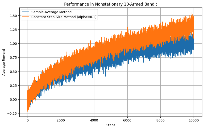
Conclusion:

This experiment demonstrates that for nonstationary problems, a constant step size provides a more appropriate adaptation mechanism than sample averages, which are more suited to stationary problems where stable estimates are desired.