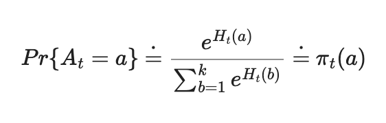
Another approach to select the most optimal action in RL problems is using the Gradient Bandit Algorithm to calculate the Relative Preferences between actions. The optimal action selection function follows the Softmax-Distribution Function

def softmax(x):
    e_x = np.exp(x - np.max(x)) 
    M = e_x / e_x.sum()
    return np.argmax(M), M

We focus on Updating Probability of Relative Preference of One Action over Other during our Optimal Action selection process.

def gradient_bandit(k, steps, alpha, initial_Q, is_baseline=True):
    rewards = np.zeros(steps)
    actions = np.zeros(steps)
    
    for i in tqdm(range(num_trials)):
        Q = np.ones(k) * initial_Q # initial Q
        N = np.zeros(k) # initalize number of rewards given
        R = np.zeros(k)
        H = np.zeros(k) # initalize preferences
        pi = np.zeros(k)
        best_action = np.argmax(q_stars[i]) # best action of i'th problem
        
        for t in range(steps):
            a, pi = softmax(H)

            reward = bandit(a, i)

            N[a] += 1
            Q[a] = Q[a] + (reward - Q[a]) / N[a]
            
            for action_i in range(k):
                if action_i == a :
                    H[a] = H[a] + alpha * (reward - R[a]) * (1 - pi[a])
                else:
                    H[action_i] = H[action_i] - alpha * (reward - R[action_i]) * pi[action_i]

            if is_baseline == True:
                R[a] = Q[a]

            rewards[t] += reward
            if a == best_action:
                actions[t] += 1
    
    return np.divide(rewards,num_trials), np.divide(actions,num_trials)

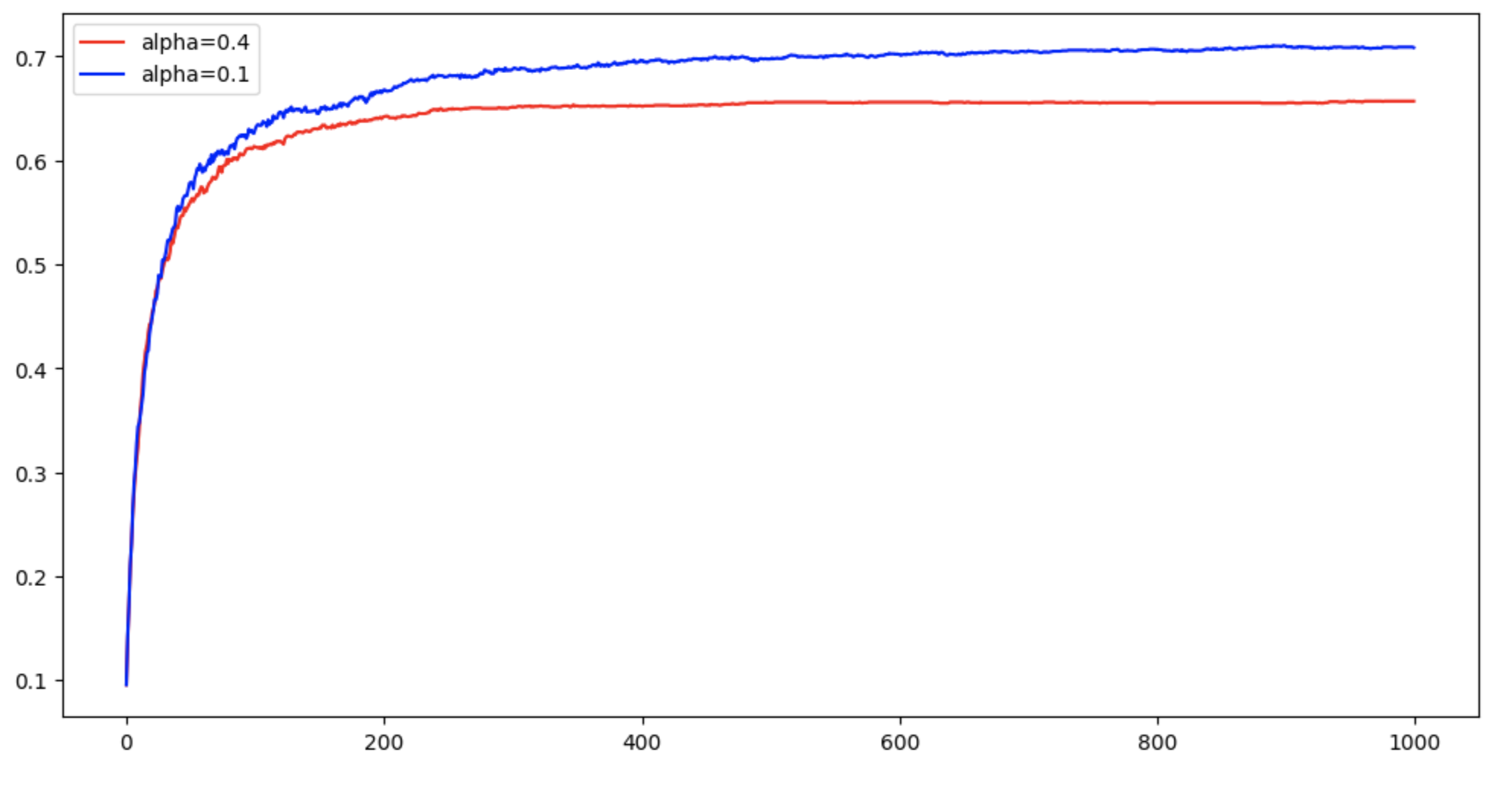
Alpha of 0.1 Performs better than Alpha of 0.4

sft_4_baseline, ac_sft_4_baseline = gradient_bandit(k=10, steps=1000, alpha=0.4, initial_Q=0, is_baseline=True)
sft_1_baseline, ac_sft_1_baseline = gradient_bandit(k=10, steps=1000, alpha=0.1, initial_Q=0, is_baseline=True)

plt.figure(figsize=(12,6))
plt.plot(ac_sft_4_baseline, 'r', label='alpha=0.4')
plt.plot(ac_sft_1_baseline, 'b', label='alpha=0.1')
# plt.plot(ac_sft_4, 'lightcoral', label='alpha=0.4 without baseline')
plt.legend() 
plt.show()