Scikit-Learn (sk-learn) was built by South Korean and American Machine Learning engineers to speed up their daily data crunching and training ML model workflow. A typical machine learning workflow with Scikit-Learn including 4 main steps

Step 1: Data Inspection and Preprocessing

Import csv file, rename all columns to lowercase with underscore, drop null value and display summary data

df = pd.read_csv("world_happiness.csv")

df = df.rename(columns={i: "_".join(i.split(" ")).lower() for i in df.columns})
df = df.dropna()
df.info()

Cross Pair Plotting between Data Columns of our Panda dataframe and export to png

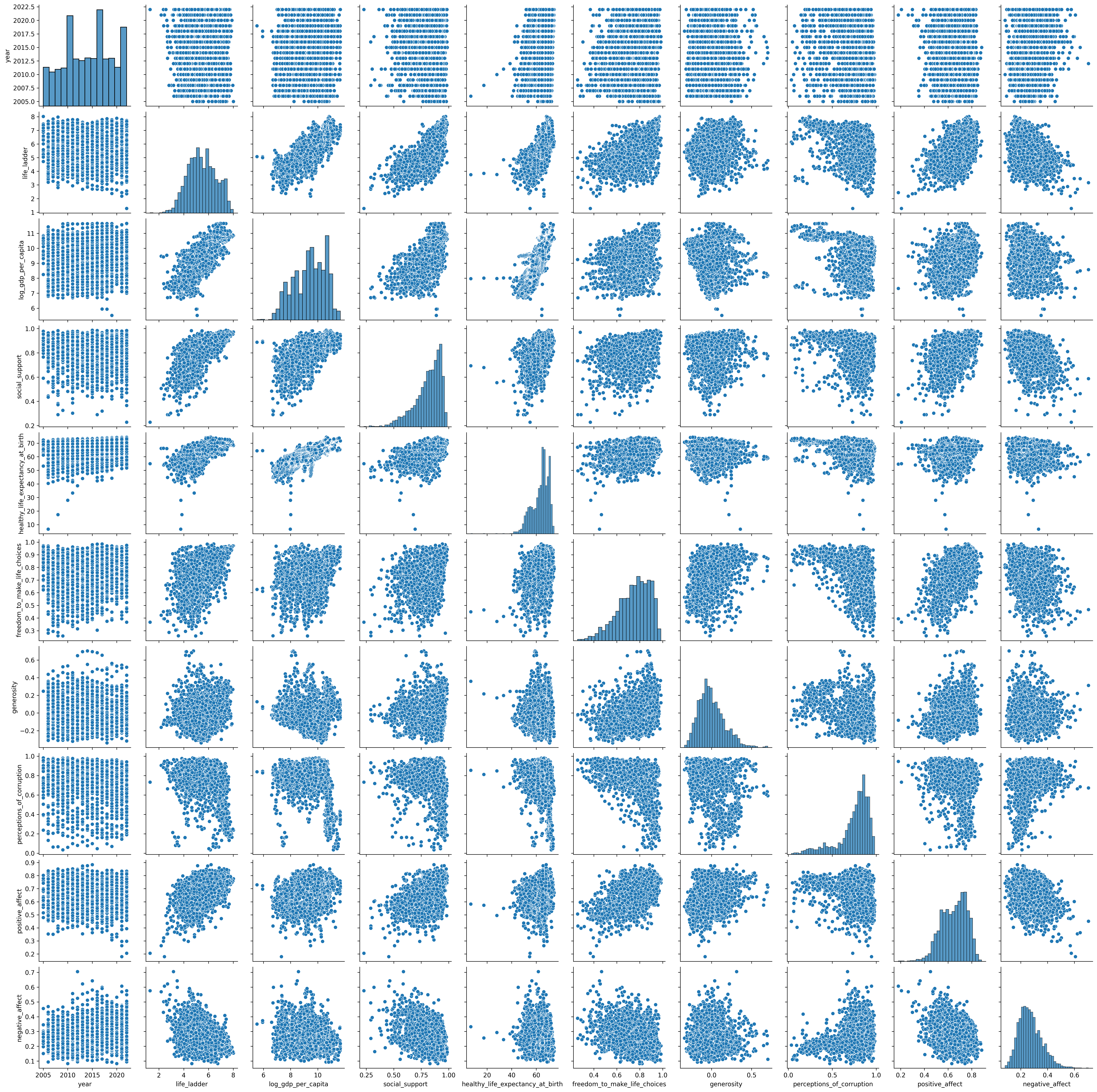
plot = sns.pairplot(df)
plot.figure.savefig("pairplot.png", dpi=300, bbox_inches='tight')

Plot of 'life_ladder' vs ['log_gdp_per_capita', 'social_support'] showing Linear Relationship between these columns. People have longer life expectancy if they have higher Income as well as more Social Supports from Friends and Family.

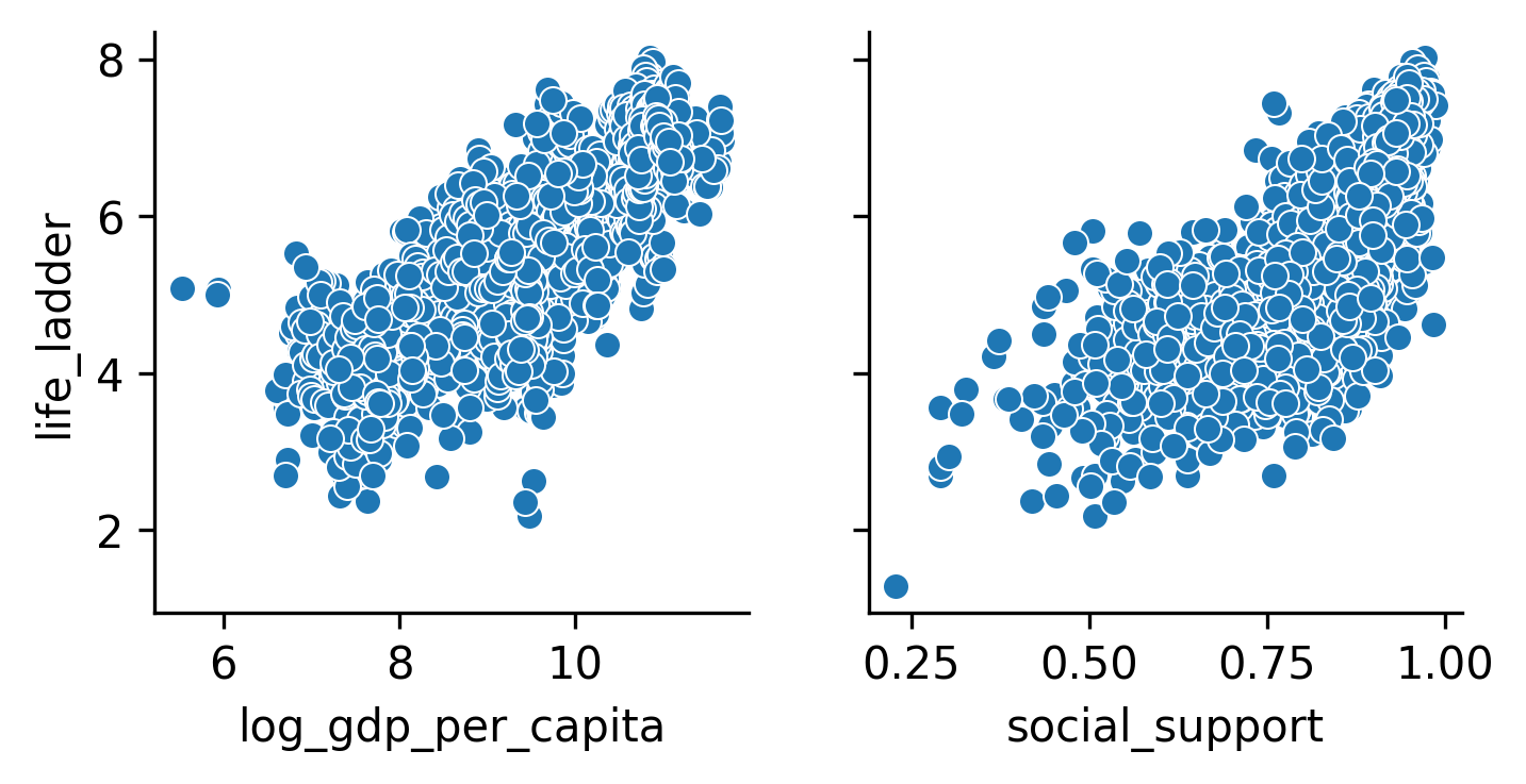
g = sns.PairGrid(
    df,
    x_vars=["log_gdp_per_capita", "social_support"],  # columns
    y_vars=["life_ladder"]                            # row
)

g.map(sns.scatterplot)
plt.show()

We also can find strong correlation between life_ladder and log_gdp_per_capita and social_support

correlations = df.corr(numeric_only=True)['life_ladder'].sort_values(ascending=False)
print(correlations)

life_ladder                         1.000000
log_gdp_per_capita                  0.784868
social_support                      0.721662
healthy_life_expectancy_at_birth    0.713499
freedom_to_make_life_choices        0.534493
positive_affect                     0.518169
generosity                          0.181630
year                                0.045947
negative_affect                    -0.339969
perceptions_of_corruption          -0.431500

Step 2: Split Data Into Test/Train Sets

We will train our Linear Regression Model weights and bias of log_gdp_per_capita and social_support after target life_ladder

X = df[['log_gdp_per_capita', 'social_support']]
y = df['life_ladder']

X_train, X_test, y_train, y_test = train_test_split(
    X, y, test_size=0.2, random_state=42
)

Step 3: Model Training with Test/Train Sets

We then fit our Linear Regression Model to the Dataset with 2 X variables log_gdp_per_capita and social_support and Y variable of life_ladder

lr = LinearRegression().fit(X_train, y_train)

We can view trained Weights and Bias of our model via lr.intercept_ and lr.coef_

b = lr.intercept_
w = lr.coef_

Weights  [0.54522093 3.14301475]
Bias  -2.174634553100434

Now we have Linear Function Formula for our Prediction as:

life_ladder = 0.54522093 * log_gdp_per_capita + 3.14301475 * social_support - 2.174634553100434

Step 4: Model Evaluation

Evaluation via Making Prediction on Test set

# Make a prediction using lr.predict()
y_test_preds = lr.predict(X_test)

# Make a prediction by hand using w, b.
y_pred = np.dot(X_test, w) + b

Calculate *** Mean Absolute Error *** and *** Relative Error*** for our Linear Regression model

### Calculate Mean Absolute Error
mae = metrics.mean_absolute_error(y_test, y_test_preds)

### Calculate Relative Error
mean_life_ladder = np.mean(y)
relative_error = mae/mean_life_ladder*100

print("Mean Absolute Error: ", mae,mean_life_ladder )
print("Relative Absolute Error: %", relative_error)

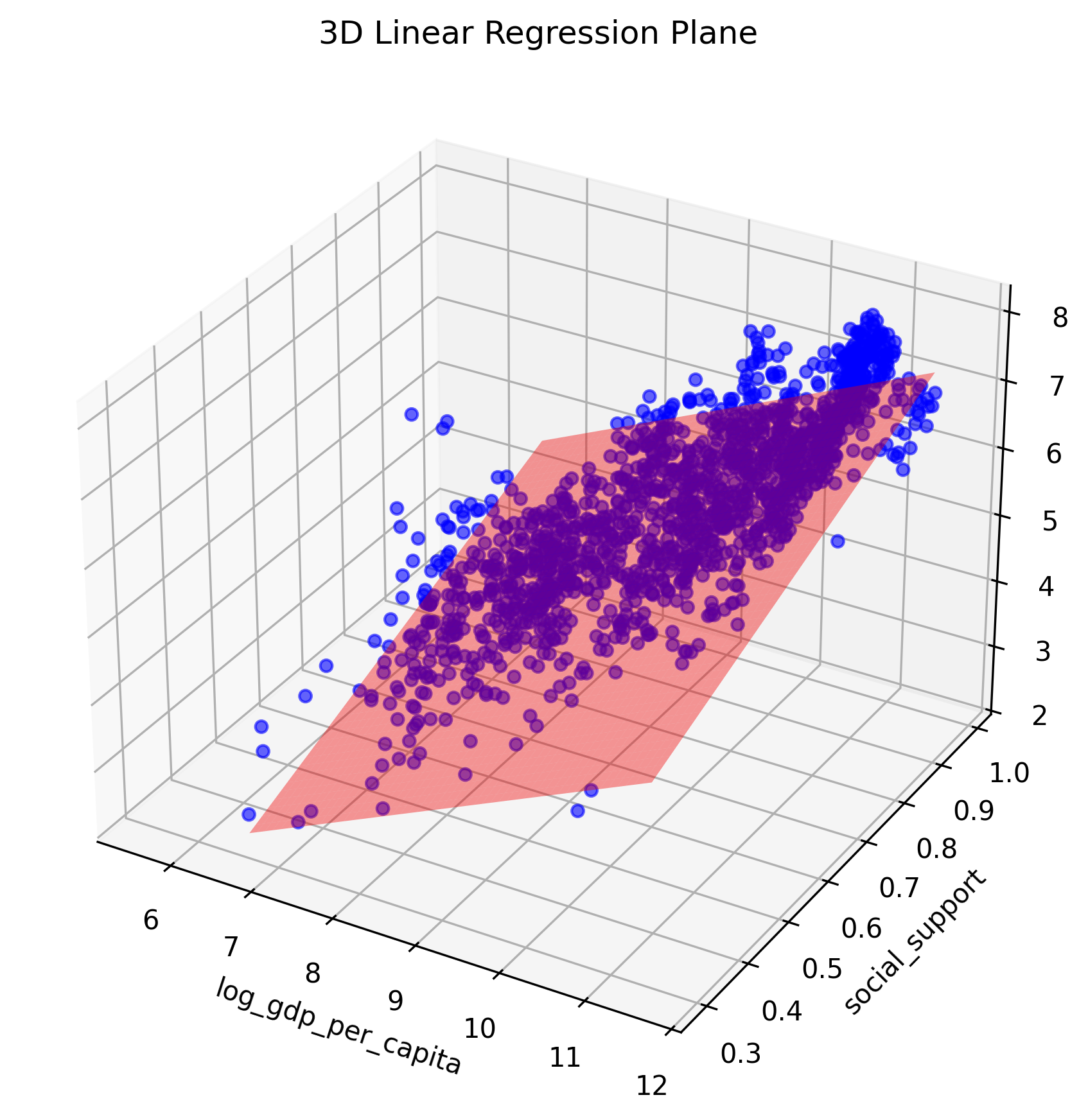
Plotting Prediction Relative to Training Data

fig = plt.figure(figsize=(10,7))
ax = fig.add_subplot(111, projection='3d')

# Plotting Training Data
ax.scatter(X_train.values[:,0], X_train.values[:,1], y_train.values, color='blue', alpha=0.6)

# Plotting Prediction Surface
x_surf, y_surf = np.meshgrid(
    np.linspace(X_test.values[:,0].min(), X_test.values[:,0].max(), 50),
    np.linspace(X_test.values[:,1].min(), X_test.values[:,1].max(), 50)
)

z_pred = model.predict(
    np.c_[x_surf.ravel(), y_surf.ravel()]
).reshape(x_surf.shape)

ax.plot_surface(
    x_surf, 
    y_surf, 
    z_pred, 
    color='red', 
    alpha=0.4
)

ax.set_xlabel('log_gdp_per_capita')
ax.set_ylabel('social_support')
ax.set_zlabel('life_ladder')
ax.set_title('3D Linear Regression Plane')

plt.savefig("Two_Features_Regression_Model.png", dpi=300, bbox_inches='tight')
plt.show()